
15. Deep Learning
Objectives
In this chapter you’ll:
![]() Understand what a neural network is and how it enables deep learning.
Understand what a neural network is and how it enables deep learning.
![]() Create Keras neural networks.
Create Keras neural networks.
![]() Understand Keras layers, activation functions, loss functions and optimizers.
Understand Keras layers, activation functions, loss functions and optimizers.
![]() Use a Keras convolutional neural network (CNN) trained on the MNIST dataset to recognize handwritten digits.
Use a Keras convolutional neural network (CNN) trained on the MNIST dataset to recognize handwritten digits.
![]() Use a Keras recurrent neural network (RNN) trained on the IMDb dataset to perform binary classification of positive and negative movie reviews.
Use a Keras recurrent neural network (RNN) trained on the IMDb dataset to perform binary classification of positive and negative movie reviews.
![]() Use TensorBoard to visualize the progress of training deep-learning networks.
Use TensorBoard to visualize the progress of training deep-learning networks.
![]() Learn which pretrained neural networks come with Keras.
Learn which pretrained neural networks come with Keras.
![]() Understand the value of using models pretrained on the massive ImageNet dataset for computer vision apps.
Understand the value of using models pretrained on the massive ImageNet dataset for computer vision apps.
Outline
15.1.1 Deep Learning Applications
15.3 Custom Anaconda Environments
15.6 Convolutional Neural Networks for Vision; Multi-Classification with the MNIST Dataset
15.6.1 Loading the MNIST Dataset
15.6.4 Creating the Neural Network
15.6.5 Training and Evaluating the Model
15.6.6 Saving and Loading a Model
15.7 Visualizing Neural Network Training with TensorBoard
15.8 ConvnetJS: Browser-Based Deep-Learning Training and Visualization
15.9 Recurrent Neural Networks for Sequences; Sentiment Analysis with the IMDb Dataset
15.9.1 Loading the IMDb Movie Reviews Dataset
15.9.4 Creating the Neural Network
15.9.5 Training and Evaluating the Model
15.10 Tuning Deep Learning Models
15.1 Introduction
One of AI’s most exciting areas is deep learning, a powerful subset of machine learning that has produced impressive results in computer vision and many other areas over the last few years. The availability of big data, significant processor power, faster Internet speeds and advancements in parallel computing hardware and software are making it possible for more organizations and individuals to pursue resource-intensive deep-learning solutions.
Keras and TensorFlow
In the previous chapter, Scikit-learn enabled you to define machine-learning models conveniently with one statement. Deep learning models require more sophisticated setups, typically connecting multiple objects, called layers. We’ll build our deep learning models with Keras, which offers a friendly interface to Google’s TensorFlow—the most widely used deep-learning library.1 François Chollet of the Google Mind team developed Keras to make deep-learning capabilities more accessible. His book Deep Learning with Python is a must read.2 Google has thousands of TensorFlow and Keras projects underway internally and that number is growing quickly.3,4
1Keras also serves as a friendlier interface to Microsofts CNTK and the Université de Montréals Theano- (which ceased development in 2017). Other popular deep learning frameworks include Caffe (http://caffe.berkeleyvision.org/), Apache MXNet (https://mxnet.apache.org/) and PyTorch (https://pytorch.org/).
2Chollet, François. Deep Learning with Python. Shelter Island, NY: Manning Publications, 2018.
3http://theweek.com/speedreads/654463/google-more-than-1000-artificial-intelligence-projects-works.
4https://www.zdnet.com/article/google-says-exponential-growth-of-ai-is-changing-nature-of-compute/.
Models
Deep learning models are complex and require an extensive mathematical background to understand their inner workings. As we’ve done throughout the book, we’ll avoid heavy mathematics here, preferring English explanations.
Keras is to deep learning as Scikit-learn is to machine learning. Each encapsulates the sophisticated mathematics, so developers need only define, parameterize and manipulate objects. With Keras, you build your models from pre-existing components and quickly parameterize those components to your unique requirements. This is what we’ve been referring to as object-based programming throughout the book.
Experiment with Your Models
Machine learning and deep learning are empirical rather than theoretical fields. You’ll experiment with many models, tweaking them in various ways until you find the models that perform best for your applications. Keras facilitates such experimentation.
Dataset Sizes
Deep learning works well when you have lots of data, but it also can be effective for smaller datasets when combined with techniques like transfer learning5,6 and data augmentation7,8. Transfer learning uses existing knowledge from a previously trained model as the foundation for a new model. Data augmentation adds data to a dataset by deriving new data from existing data. For example, in an image dataset, you might rotate the images left and right so the model can learn about objects in different orientations. In general, though, the more data you have, the better you’ll be able to train a deep learning model.
5https://towardsdatascience.com/transfer-learning-from-pre-trained-models-f2393f124751.
6https://medium.com/nanonets/nanonets-how-to-use-deep-learning-when-you-have-limited-data-f68c0b512cab.
7https://towardsdatascience.com/data-augmentation-and-images-7aca9bd0dbe8.
8https://medium.com/nanonets/how-to-use-deep-learning-when-you-have-limited-data-part-2-data-augmentation-c26971dc8ced.
Processing Power
Deep learning can require significant processing power. Complex models trained on big-data datasets can take hours, days or even more to train. The models we present in this chapter can be trained in minutes to just less than an hour on computers with conventional CPUs. You’ll need only a reasonably current personal computer. We’ll discuss the special high-performance hardware called GPUs (Graphics Processing Units) and TPUs (Tensor Processing Units) developed by NVIDIA and Google to meet the extraordinary processing demands of edge-of-the-practice deep-learning applications.
Bundled Datasets
Keras comes packaged with some popular datasets. You’ll work with two of these datasets in the chapter’s examples. You can find many Keras studies online for each of these datasets, including ones that take different approaches.
In the “Machine Learning” chapter, you worked with Scikit-learn’s Digits dataset, which contained 1797 handwritten-digit images that were selected from the much larger MNIST dataset (60,000 training images and 10,000 test images).9 In this chapter you’ll work with the full MNIST dataset. You’ll build a Keras convolutional neural network (CNN or convnet) model that will achieve high performance recognizing digit images in the test set. Convnets are especially appropriate for computer vision tasks, such as recognizing handwritten digits and characters or recognizing objects (including faces) in images and videos. You’ll also work with a Keras recurrent neural network. In that example, you’ll perform sentiment analysis using the IMDb Movie reviews dataset, in which the reviews in the training and testing sets are labeled as positive or negative.
9The MNIST Database. MNIST Handwritten Digit Database, Yann LeCun, Corinna Cortes and Chris Burges. http://yann.lecun.com/exdb/mnist/.
Future of Deep Learning
Newer automated deep learning capabilities are making it even easier to build deep-learning solutions. These include Auto-Keras10 from Texas A&M University’s DATA Lab, Baidu’s EZDL11 and Google’s AutoML12.
12https://cloud.google.com/automl/.
15.1.1 Deep Learning Applications
Deep learning is being used in a wide range of applications, such as:
Game playing
Computer vision: Object recognition, pattern recognition, facial recognition
Self-driving cars
Robotics
Improving customer experiences
Chatbots
Diagnosing medical conditions
Google Search
Facial recognition
Automated image captioning and video closed captioning
Enhancing image resolution
Speech recognition
Language translation
Predicting election results
Predicting earthquakes and weather
Google Sunroof to determine whether you can put solar panels on your roof
Generative applications—Generating original images, processing existing images to look like a specified artist’s style, adding color to black-and-white images and video, creating music, creating text (books, poetry) and much more.
15.1.2 Deep Learning Demos
Check out these four deep-learning demos and search online for lots more, including practical applications like we mentioned in the preceding section:
DeepArt.io—Turn a photo into artwork by applying an art style to the photo.
https://deepart.io/.DeepWarp Demo—Analyzes a person’s photo and makes the person’s eyes move in different directions.
https://sites.skoltech.ru/sites/compvision_wiki/static_pages/projects/deepwarp/.Image-to-Image Demo—Translates a line drawing into a picture.
https://affinelayer.com/pixsrv/.Google Translate Mobile App (download from an app store to your smartphone)—Translate text in a photo to another language (e.g., take a photo of a sign or a restaurant menu in Spanish and translate the text to English).
15.1.3 Keras Resources
Here are some resources you might find valuable as you study deep learning:
To get your questions answered, go to the Keras team’s slack channel at
https://kerasteam.slack.com.For articles and tutorials, visit
https://blog.keras.io.The Keras documentation is at
http://keras.io.If you’re looking for term projects, directed study projects, capstone course projects or thesis topics, visit arXiv (pronounced “archive,” where the X represents the Greek letter “chi”) at
https://arXiv.org. People post their research papers here in parallel with going through peer review for formal publication, hoping for fast feedback. So, this site gives you access to extremely current research.
15.2 Keras Built-In Datasets
Here are some of Keras’s datasets (from the module tensorflow.keras.datasets13) for practicing deep learning. We’ll use a couple of these in the chapter’s examples:
13In the standalone Keras library, the module names begin with keras rather than tensorflow.keras.
MNIST14 database of handwritten digits—Used for classifying handwritten digit images, this dataset contains 28-by-28 grayscale digit images labeled as 0 through 9 with 60,000 images for training and 10,000 for testing. We use this dataset in Section 15.6, where we study convolutional neural networks.
14The MNIST Database. MNIST Handwritten Digit Database, Yann LeCun, Corinna Cortes and Chris Burges.
http://yann.lecun.com/exdb/mnist/.Fashion-MNIST15 database of fashion articles—Used for classifying clothing images, this dataset contains 28-by-28 grayscale images of clothing labeled in 10 categories16 with 60,000 for training and 10,000 for testing. Once you build a model for use with MNIST, you can reuse that model with Fashion-MNIST by changing a few statements.
IMDb Movie reviews17—Used for sentiment analysis, this dataset contains reviews labeled as positive (1) or negative (0) sentiment with 25,000 reviews for training and 25,000 for testing. We use this dataset in Section 15.9, where we study recurrent neural networks.
15Han Xiao and Kashif Rasul and Roland Vollgraf, Fashion-MNIST: a Novel Image Dataset for Benchmarking Machine Learning Algorithms, arXiv, cs.LG/1708.07747.
16
https://keras.io/datasets/#fashion-mnist-database-of-fashion-articles.17Andrew L. Maas, Raymond E. Daly, Peter T. Pham, Dan Huang, Andrew Y. Ng, and Christopher Potts. (2011). Learning Word Vectors for Sentiment Analysis. The 49th Annual Meeting of the Association for Computational Linguistics (ACL 2011).
CIFAR1018 small image classification—Used for small-image classification, this dataset contains 32-by-32 color images labeled in 10 categories with 50,000 images for training and 10,000 for testing.
CIFAR10019 small image classification—Also, used for small-image classification, this dataset contains 32-by-32 color images labeled in 100 categories with 50,000 images for training and 10,000 for testing.
15.3 Custom Anaconda Environments
Before running this chapter’s examples, you’ll need to install the libraries we use. In this chapter’s examples, we’ll use the TensorFlow deep-learning library’s version of Keras.20 At the time of this writing, TensorFlow does not yet support Python 3.7. So, you’ll need Python 3.6.x to execute this chapter’s examples. We’ll show you how to set up a custom environment for working with Keras and TensorFlow.
20Theres also a standalone version that enables you to choose between TensorFlow, Microsofts CNTK or the Université de Montréals Theano (which ceased development in 2017).
Environments in Anaconda
The Anaconda Python distribution makes it easy to create custom environments. These are separate configurations in which you can install different libraries and different library versions. This can help with reproducibility if your code depends on specific Python or library versions.21
21In the next chapter, well introduce Docker as another reproducibility mechanism and as a convenient way to install complex environments for use on your local computer.
The default environment in Anaconda is called the base environment. This is created for you when you install Anaconda. All the Python libraries that come with Anaconda are installed into the base environment and, unless you specify otherwise, any additional libraries you install also are placed there. Custom environments give you control over the specific libraries you wish to install for your specific tasks.
Creating an Anaconda Environment
The conda create command creates an environment. Let’s create a TensorFlow environment and name it tf_env (you can name it whatever you like). Run the following command in your Terminal, shell or Anaconda Command Prompt:22,23
22Windows users should run the Anaconda Command Prompt as Administrator,
23If you have a computer with an NVIDIA GPU thats compatible with TensorFlow, you can replace the tensorflow library with tensorflow-gpu to get better performance. For more information, see https://www.tensorflow.org/install/gpu. Some AMD GPUs also can be used with TensorFlow: http://timdettmers.com/2018/11/05/which-gpu-for-deep-learning/.
conda create -n tf_env tensorflow anaconda ipython jupyterlab scikit-learn matplotlib seaborn h5py pydot graphviz
This will determine the listed libraries’ dependencies, then display all the libraries that will be installed in the new environment. There are many dependencies, so this may take a few minutes. When you see the prompt:
Proceed ([y]/n)?
press Enter to create the environment and install the libraries.24
24When we created our custom environment, conda installed Python 3.6.7, which was the most recent Python version compatible with the tensorflow library.
Activating an Alternate Anaconda Environment
To use a custom environment, execute the conda activate command:
conda activate tf_env
This affects only the current Terminal, shell or Anaconda Command Prompt. When a custom environment is activated and you install more libraries, they become part of the activated environment, not the base environment. If you open separate Terminals, shells or Anaconda Command Prompts, they’ll use Anaconda’s base environment by default.
Deactivating an Alternate Anaconda Environment
When you’re done with a custom environment, you can return to the base environment in the current Terminal, shell or Anaconda Command Prompt by executing:
conda deactivate
Jupyter Notebooks and JupyterLab
This chapter’s examples are provided only as Jupyter Notebooks, which will make it easier for you to experiment with the examples. You can tweak the options we present and reexecute the notebooks. For this chapter, you should launch JupyterLab from the ch15 examples folder (as discussed in Section 1.5.3).
15.4 Neural Networks
Deep learning is a form of machine learning that uses artificial neural networks to learn. An artificial neural network (or just neural network) is a software construct that operates similarly to how scientists believe our brains work. Our biological nervous systems are controlled via neurons25 that communicate with one another along pathways called synapses26. As we learn, the specific neurons that enable us to perform a given task, like walking, communicate with one another more efficiently. These neurons activate anytime we need to walk.27
25https://en.wikipedia.org/wiki/Neuron.
26https://en.wikipedia.org/wiki/Synapse.
27https://www.sciencenewsforstudents.org/article/learning-rewires-brain.
Artificial Neurons
In a neural network, interconnected artificial neurons simulate the human brain’s neurons to help the network learn. The connections between specific neurons are reinforced during the learning process with the goal of achieving a specific result. In supervised deep learning—which we’ll use in this chapter—we aim to predict the target labels supplied with data samples. To do this, we’ll train a general neural network model that we can then use to make predictions on unseen data.28
28As in machine learning, you can create unsupervised deep learning networksthese are beyond this chapters scope.
Artificial Neural Network Diagram
The following diagram shows a three-layer neural network. Each circle represents a neuron, and the lines between them simulate the synapses. The output of a neuron becomes the input of another neuron, hence the term neural network. This particular diagram shows a fully connected network—every neuron in a given layer is connected to all the neurons in the next layer:

Learning Is an Iterative Process
When you were a baby, you did not learn to walk instantaneously. You learned that process over time with repetition. You built up the smaller components of the movements that enabled you to walk—learning to stand, learning to balance to remain standing, learning to lift your foot and move it forward, etc. And you got feedback from your environment. When you walked successfully your parents smiled and clapped. When you fell, you might have bumped your head and felt pain.
Similarly, we train neural networks iteratively over time. Each iteration is known as an epoch and processes every sample in the training dataset once. There’s no “correct” number of epochs. This is a hyperparameter that may need tuning, based on your training data and your model. The inputs to the network are the features in the training samples. Some layers learn new features from previous layers’ outputs and others interpret those features to make predictions.
How Artificial Neurons Decide Whether to Activate Synapses
During the training phase, the network calculates values called weights for every connection between the neurons in one layer and those in the next. On a neuron-by-neuron basis, each of its inputs is multiplied by that connection’s weight, then the sum of those weighted inputs is passed to the neuron’s activation function. This function’s output determines which neurons to activate based on the inputs—just like the neurons in your brain passing information around in response to inputs coming from your eyes, nose, ears and more. The following diagram shows a neuron receiving three inputs (the black dots) and producing an output (the hollow circle) that would be passed to all or some of neurons in the next layer, depending on the types of the neural network’s layers:

The values w1, w2 and w3 are weights. In a new model that you train from scratch, these values are initialized randomly by the model. As the network trains, it tries to minimize the error rate between the network’s predicted labels and the samples’ actual labels. The error rate is known as the loss, and the calculation that determines the loss is called the loss function. Throughout training, the network determines the amount that each neuron contributes to the overall loss, then goes back through the layers and adjusts the weights in an effort to minimize that loss. This technique is called backpropagation. Optimizing these weights occurs gradually—typically via a process called gradient descent.
15.5 Tensors
Deep learning frameworks generally manipulate data in the form of tensors. A “tensor” is basically a multidimensional array. Frameworks like TensorFlow pack all your data into one or more tensors, which they use to perform the mathematical calculations that enable neural networks to learn. These tensors can become quite large as the number of dimensions increases and as the richness of the data increases (for example, images, audios and videos are richer than text). Chollet discusses the types of tensors typically encountered in deep learning:29
29Chollet, François. Deep Learning with Python. Section 2.2. Shelter Island, NY: Manning Publications, 2018.
0D (0-dimensional) tensor—This is one value and is known as a scalar.
1D tensor—This is similar to a one-dimensional array and is known as a vector. A 1D tensor might represent a sequence, such as hourly temperature readings from a sensor or the words of one movie review.
2D tensor—This is similar to a two-dimensional array and is known as a matrix. A 2D tensor could represent a grayscale image in which the tensor’s two dimensions are the image’s width and height in pixels, and the value in each element is the intensity of that pixel.
3D tensor—This is similar to a three-dimensional array and could be used to represent a color image. The first two dimensions would represent the width and height of the image in pixels and the depth at each location might represent the red, green and blue (RGB) components of a given pixel’s color. A 3D tensor also could represent a collection of 2D tensors containing grayscale images.
4D tensor—A 4D tensor could be used to represent a collection of color images in 3D tensors. It also could be used to represent one video. Each frame in a video is essentially a color image.
5D tensor—This could be used to represent a collection of 4D tensors containing videos.
A tensor’s shape typically is represented as a tuple of values in which the number of elements specifies the tensor’s number of dimensions and each value in the tuple specifies the size of the tensor’s corresponding dimension.
Let’s assume we’re creating a deep-learning network to identify and track objects in 4K (high-resolution) videos that have 30 frames-per-second. Each frame in a 4K video is 3840-by-2160 pixels. Let’s also assume the pixels are presented as red, green and blue components of a color. So each frame would be a 3D tensor containing a total of 24,883,200 elements (3840 * 2160 * 3) and each video would be a 4D tensor containing the sequence of frames. If the videos are one minute long, you’d have 44,789,760,000 elements per tensor!
Over 600 hours of video are uploaded to YouTube every minute30 so, in just one minute of uploads, Google could have a tensor containing 1,612,431,360,000,000 elements to use in training deep-learning models—that’s big data. As you can see, tensors can quickly become enormous, so manipulating them efficiently is crucial. This is one of the key reasons that most deep learning is performed on GPUs. More recently Google created TPUs (Tensor Processing Units) that are specifically designed to perform tensor manipulations, executing faster than GPUs.
30https://www.inc.com/tom-popomaronis/youtube-analyzed-trillions-of-data-points-in-2018-revealing-5-eye-opening-behavioral-statistics.html.
High-Performance Processors
Powerful processors are needed for real-world deep learning because the size of tensors can be enormous and large-tensor operations can place crushing demands on processors. The processors most commonly used for deep learning are:
NVIDIA GPUs (Graphics Processing Units)—Originally developed by companies like NVIDIA for computer gaming, GPUs are much faster than conventional CPUs for processing large amounts of data, thus enabling developers to train, validate and test deep-learning models more efficiently—and thus experiment with more of them. GPUs are optimized for the mathematical matrix operations typically performed on tensors, an essential aspect of how deep learning works “under the hood.” NVIDIA’s Volta Tensor Cores are specifically designed for deep learning.31,32 Many NVIDIA GPUs are compatible with TensorFlow, and hence Keras, and can enhance the performance of your deep-learning models.33
31
https://www.nvidia.com/en-us/data-center/tensorcore/.32
https://devblogs.nvidia.com/tensor-core-ai-performance-milestones/.Google TPUs (Tensor Processing Units)—Recognizing that deep learning is crucial to its future, Google developed TPUs (Tensor Processing Units), which they now use in their Cloud TPU service, which “can provide up to 11.5 petaflops of performance in a single pod”34 (that’s 11.5 quadrillion floating-point operations per second). Also, TPUs are designed to be especially energy efficient. This is a key concern for companies like Google with already massive computing clusters that are growing exponentially and consuming vast amounts of energy.
15.6 Convolutional Neural Networks for Vision; Multi-Classification with the MNIST Dataset
In the “Machine Learning” chapter, we classified handwritten digits using the 8-by-8-pixel, low-resolution images from the Digits dataset bundled with Scikit-learn. That dataset is based on a subset of the higher-resolution MNIST handwritten digits dataset. Here, we’ll use MNIST to explore deep learning with a convolutional neural network35 (also called a convnet or CNN). Convnets are common in computer-vision applications, such as recognizing handwritten digits and characters, and recognizing objects in images and video. They’re also used in non-vision applications, such as natural-language processing and recommender systems.
35https://en.wikipedia.org/wiki/Convolutional_neural_network.
The Digits dataset has only 1797 samples, whereas MNIST has 70,000 labeled digit image samples—60,000 for training and 10,000 for testing. Each sample is a grayscale 28-by-28 pixel image (784 total features) represented as a NumPy array. Each pixel is a value from 0 to 255 representing the intensity (or shade) of that pixel—the Digits dataset uses less granular shading with values from 0 to 16. MNIST’s labels are integer values in the range 0 through 9, indicating the digit each image represents.
The machine-learning model you used in the previous chapter produced as its output a digit image’s predicted class—an integer in the range 0–9. The convnet model we’ll build will perform probabilistic classification.36 For each digit image, the model will output an array of 10 probabilities, each indicating the likelihood that the digit belongs to a particular one of the classes 0 through 9. The class with the highest probability is the predicted value.
36https://en.wikipedia.org/wiki/Probabilistic_classification.
Reproducibility in Keras and Deep Learning
We’ve discussed the importance of reproducibility throughout the book. In deep learning, reproducibility is more difficult because the libraries heavily parallelize operations that perform floating-point calculations. Each time operations execute, they may execute in a different order. This can produce differences in your results. Getting reproducible results in Keras requires a combination of environment settings and code settings that are described in the Keras FAQ:
https://keras.io/getting-started/faq/#how-can-i-obtain-reproducible-results-using-keras-during-development
Basic Keras Neural Network
A Keras neural network consists of the following components:
A network (also called a model)—A sequence of layers containing the neurons used to learn from the samples. Each layer’s neurons receive inputs, process them (via an activation function) and produce outputs. The data is fed into the network via an input layer that specifies the dimensions of the sample data. This is followed by hidden layers of neurons that implement the learning and an output layer that produces the predictions. The more layers you stack, the deeper the network is, hence the term deep learning.
A loss function—This produces a measure of how well the network predicts the target values. Lower loss values indicate better predictions.
An optimizer—This attempts to minimize the values produced by the loss function to tune the network to make better predictions.
Launch JupyterLab
This section assumes that you’ve activated the tf_env Anaconda environment you created in Section 15.3 and launched JupyterLab from the ch15 examples folder. You can either open the MNIST_CNN.ipynb file in JupyterLab and execute the code in the cells we provided, or you can create a new notebook and enter the code on your own. If you prefer, you can work at the command line in IPython, however, placing your code in a Jupyter Notebook makes it significantly easier for you to re-execute this chapter’s examples.
As a reminder, you can reset a Jupyter Notebook and remove its outputs by selecting Restart Kernel and Clear All Outputs from JupyterLab’s Kernel menu. This terminates the notebook’s execution and removes its outputs. You might do this if your model is not performing well and you want to try different hyperparameters or possibly restructure your neural network.37 You can then re-execute the notebook one cell at a time or execute the entire notebook by selecting Run All from JupyterLab’s Run menu.
37We found that we sometimes had to execute this menu option twice to clear the outputs.
15.6.1 Loading the MNIST Dataset
Let’s import the tensorflow.keras.datasets.mnist module so we can load the dataset:
[1]:fromtensorflow.keras.datasetsimportmnist
Note that because we’re using the version of Keras built into TensorFlow, the Keras module names begin with "tensorflow.". In the standalone Keras version, the module names begin with "keras.", so keras.datasets would be used above. Keras uses TensorFlow to execute the deep-learning models.
The mnist module’s load_data function loads the MNIST training and testing sets:
[2]: (X_train, y_train), (X_test, y_test) = mnist.load_data()
When you call load_data it will download the MNIST data to your system. The function returns a tuple of two elements containing the training and testing sets. Each element is itself a tuple containing the samples and labels, respectively.
15.6.2 Data Exploration
Let’s get to know the data before working with it. First, we check the dimensions of the training set images (X_train), training set labels (y_train), testing set images (X_test) and testing set labels (y_test):
[3]: X_train.shape
[3]: (60000, 28, 28)

[4]: y_train.shape
[4]: (60000,)

[5]: X_test.shape
[5]: (10000, 28, 28)

[6]: y_test.shape
[6]: (10000,)
You can see from X_train’s and X_test’s shapes that the images are higher resolution than those in Scikit-learn’s Digits dataset (which are 8-by-8).
Visualizing Digits
Let’s visualize some of the digit images. First, enable Matplotlib in the notebook, import Matplotlib and Seaborn and set the font scale:
[7]: %matplotlib inline [8]:importmatplotlib.pyplotasplt [9]:importseabornassns [10]: sns.set(font_scale=2)
The IPython magic
%matplotlib inline
indicates that Matplotlib-based graphics should be displayed in the notebook rather than in separate windows. For more IPython magics, you can use in Jupyter Notebooks, see:
https://ipython.readthedocs.io/en/stable/interactive/magics.html
Next, we’ll display a randomly selected set of 24 MNIST training set images. Recall from the “Array-Oriented Programming with NumPy” chapter that you can pass a sequence of indexes as a NumPy array’s subscript to select only the array elements at those indexes. We’ll use that capability here to select the elements at the same indexes in both the X_train and y_train arrays. This ensures that we display the correct label for each randomly selected image.
NumPy’s choice function (from the numpy.random module) randomly selects the number of elements specified in its second argument (24) from the array of values in its first argument (in this case, an array containing X_train’s range of indices). The function returns an array containing the selected values, which we store in index. The expressions X_train[index] and y_train[index] use index to get the corresponding elements from both arrays. The rest of this cell is the visualization code from the previous chapter’s Digits case study:
[11]:importnumpyasnp index = np.random.choice(np.arange(len(X_train)),24, replace=False) figure, axes = plt.subplots(nrows=4, ncols=6, figsize=(16,9))foriteminzip(axes.ravel(), X_train[index], y_train[index]): axes, image, target = item axes.imshow(image, cmap=plt.cm.gray_r) axes.set_xticks([])# remove x-axis tick marksaxes.set_yticks([])# remove y-axis tick marksaxes.set_title(target) plt.tight_layout()
You can see in the output below that MNIST’s digit images have higher resolution than those in Scikit-learn’s Digits dataset.
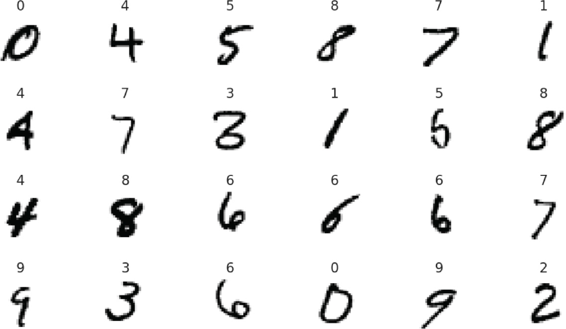
Looking at the digits, you can see why handwritten digit recognition is a challenge:
Some people write “open” 4s (like the ones in the first and third rows), and some write “closed” 4s (like the one in the second row). Though each 4 has some similar features, they’re all different from one another.
The 3 in the second row looks strange—more like a merged 6 and 7. Compare this to the much clearer 3 in the fourth row.
The 5 in the second row could easily be confused with a 6.
Also, people write their digits at different angles, as you can see with the four 6s in the third and fourth rows—two are upright, one leans left and one leans right.
If you run the preceding snippet multiple times, you can see additional randomly selected digits.38 You’ll probably find that—if not for the labels displayed above each digit—it would be difficult for you to identify some of the digits. We’ll soon see how accurately our first convnet will predict the digits in the MNIST test set.
38If you do run the cell multiple times, the snippet number next to the cell will increment each time, as it does in IPython at the command line.
15.6.3 Data Preparation
Recall from the “Machine Learning” chapter that Scikit-learn’s bundled datasets were preprocessed into the shapes its models required. In real-world studies, you’ll generally have to do some or all of the data preparation. The MNIST dataset requires some preparation for use in a Keras convnet.
Reshaping the Image Data
Keras convnets require NumPy array inputs in which each sample has the shape:
(width, height, channels)
For MNIST, each image’s width and height are 28 pixels, and each pixel has one channel (the grayscale shade of the pixel from 0 to 255), so each sample’s shape will be:
(28, 28, 1)
Full-color images with RGB (red/green/blue) values for each pixel, would have three channels—one channel each for the red, green and blue components of a color.
As the neural network learns from the images, it creates many more channels. Rather than shade or color, the learned channels will represent more complex features, like edges, curves and lines, that will eventually enable the network to recognize digits based on these additional features and how they’re combined.
Let’s reshape the 60,000 training and 10,000 testing set images into the correct dimensions for use in our convnet and confirm their new shapes. Recall that NumPy array method reshape receives a tuple representing the array’s new shape:
[12]: X_train = X_train.reshape((60000,28,28,1)) [13]: X_train.shape [13]: (60000, 28, 28, 1) [14]: X_test = X_test.reshape((10000,28,28,1)) [15]: X_test.shape [15]: (10000, 28, 28, 1)
Normalizing the Image Data
Numeric features in data samples may have value ranges that vary widely. Deep learning networks perform better on data that is scaled either into the range 0.0 to 1.0, or to a range for which the data’s mean is 0.0 and its standard deviation is 1.0.39 Getting your data into one of these forms is known as normalization.
39S. Ioffe and Szegedy, C.. Batch Normalization: Accelerating Deep Network Training by Reducing Internal Covariate Shift. https://arxiv.org/abs/1502.03167.
In MNIST, each pixel is an integer in the range 0–255. The following statements convert the values to 32-bit (4-byte) floating-point numbers using the NumPy array method astype, then divide every element in the resulting array by 255, producing normalized values in the range 0.0–1.0:
[16]: X_train = X_train.astype('float32') /255[17]: X_test = X_test.astype('float32') /255
One-Hot Encoding: Converting the Labels From Integers to Categorical Data
As we mentioned, the convnet’s prediction for each digit will be an array of 10 probabilities, indicating the likelihood that the digit belongs to a particular one of the classes 0 through 9. When we evaluate the model’s accuracy, Keras compares the model’s predictions to the labels. To do that, Keras requires both to have the same shape. The MNIST label for each digit, however, is one integer value in the range 0–9. So, we must transform the labels into categorical data—that is, arrays of categories that match the format of the predictions. To do this, we’ll use a process called one-hot encoding,40 which converts data into arrays of 1.0s and 0.0s in which only one element is 1.0 and the rest are 0.0s. For MNIST, the one-hot-encoded values will be 10-element arrays representing the categories 0 through 9. One-hot encoding also can be applied to other types of data.
40This term comes from certain digital circuits in which a group of bits is allowed to have only one bit turned on (that is, to have the value 1). https://en.wikipedia.org/wiki/One-hot.
We know precisely which category each digit belongs to, so the categorical representation of a digit label will consist of a 1.0 at that digit’s index and 0.0s for all the other elements (again, Keras uses floating-point numbers internally). So, a 7’s categorical representation is:
[0.0, 0.0, 0.0, 0.0, 0.0, 0.0, 0.0, 1.0, 0.0, 0.0]
and a 3’s representation is:
[0.0, 0.0, 0.0, 1.0, 0.0, 0.0, 0.0, 0.0, 0.0, 0.0]
The tensorflow.keras.utils module provides function to_categorical to perform one-hot encoding. The function counts the unique categories then, for each item being encoded, creates an array of that length with a 1.0 in the correct position. Let’s transform y_train and y_test from one-dimensional arrays containing the values 0–9 into two-dimensional arrays of categorical data. After doing so, the rows of these arrays will look like those shown above. Snippet [21] outputs one sample’s categorical data for the digit 5 (recall that NumPy shows the decimal point, but not trailing 0s on floating-point values):
[18]:fromtensorflow.keras.utilsimportto_categorical [19]: y_train = to_categorical(y_train) [20]: y_train.shape [20]: (60000, 10) [21]: y_train[0] [21]: array([ 0., 0., 0., 0., 0., 1., 0., 0., 0., 0.], dtype=float32) [22]: y_test = to_categorical(y_test) [23]: y_test.shape [23]: (10000, 10)
15.6.4 Creating the Neural Network
Now that we’ve prepared the data, we’ll configure a convolutional neural network. We begin with the Keras Sequential model from the tensorflow.keras.models module:
[24]:fromtensorflow.keras.modelsimportSequential [25]: cnn = Sequential()
The resulting network will execute its layers sequentially—the output of one layer becomes the input to the next. This is known as a feed-forward network. As you’ll see when we discuss recurrent neural networks, not all neural network operate this way.
Adding Layers to the Network
A typical convolutional neural network consists of several layers—an input layer that receives the training samples, hidden layers that learn from the samples and an output layer that produces the prediction probabilities. We’ll create a basic convnet here. Let’s import from the tensorflow.keras.layers module the layer classes we’ll use in this example:
[26]:fromtensorflow.keras.layersimportConv2D, Dense, Flatten,
MaxPooling2D-
We discuss each below.
Convolution
We’ll begin our network with a convolution layer, which uses the relationships between pixels that are close to one another to learn useful features (or patterns) in small areas of each sample. These features become inputs to subsequent layers.
The small areas that convolution learns from are called kernels or patches. Let’s examine convolution on a 6-by-6 image. Consider the following diagram in which the 3-by-3 shaded square represents the kernel—the numbers are simply position numbers showing the order in which the kernels are visited and processed:

The small areas that convolution learns from are called kernels or patches. Let’s examine convolution on a 6-by-6 image. Consider the following diagram in which the 3-by-3 shaded square represents the kernel—the numbers are simply position numbers showing the order in which the kernels are visited and processed:
You can think of the kernel as a “sliding window” that the convolution layer moves one pixel at a time left-to-right across the image. When the kernel reaches the right edge, the convolution layer moves the kernel one pixel down and repeats this left-to-right process. Kernels typically are 3-by-3,41 though we found convnets that used 5-by-5 and 7-by-7 for higher-resolution images. Kernel-size is a tunable hyperparameter.
41https://www.quora.com/How-can-I-decide-the-kernel-size-output-maps-and-layers-of-CNN.
Initially, the kernel is in the upper-left corner of the original image—kernel position 1 (the shaded square) in the input layer above. The convolution layer performs mathematical calculations using those nine features to “learn” about them, then outputs one new feature to position 1 in the layer’s output. By looking at features near one another, the network begins to recognize features like edges, straight lines and curves.
Next, the convolution layer moves the kernel one pixel to the right (known as the stride) to position 2 in the input layer. This new position overlaps with two of the three columns in the previous position, so that the convolution layer can learn from all the features that touch one another. The layer learns from the nine features in kernel position 2 and outputs one new feature in position 2 of the output, as in:

For a 6-by-6 image and a 3-by-3 kernel, the convolution layer does this two more times to produce features for positions 3 and 4 of the layer’s output. Then, the convolution layer moves the kernel one pixel down and begins the left-to-right process again for the next four kernel positions, producing outputs in positions 5–8, then 9–12 and finally 13–16. The complete pass of the image left-to-right and top-to-bottom is called a filter. For a 3-by-3 kernel, the filter dimensions (4-by-4 in our sample above) will be two less than the input dimensions (6-by-6). For each 28-by-28 MNIST image, the filter will be 26-by-26.
The number of filters in the convolutional layer is commonly 32 or 64 when processing small images like those in MNIST, and each filter produces different results. The number of filters depends on the image dimensions—higher-resolution images have more features, so they require more filters. If you study the code the Keras team used to produce their pretrained convnets,42 you’ll find that they used 64, 128 or even 256 filters in their first convolutional layers. Based on their convnets and the fact that the MNIST images are small, we’ll use 64 filters in our first convolutional layer. The set of filters produced by a convolution layer is called a feature map.
42https://github.com/keras-team/keras-applications/tree/master/keras_applications.
Subsequent convolution layers combine features from previous feature maps to recognize larger features and so on. If we were doing facial recognition, early layers might recognize lines, edges and curves, and subsequent layers might begin combining those into larger features like eyes, eyebrows, noses, ears and mouths. Once the network learns a feature, because of convolution, it can recognize that feature anywhere in the image. This is one of the reasons that convnets are used for object recognition in images.
Adding a Convolution Layer
Let’s add a Conv2D convolution layer to our model:
[27]: cnn.add(Conv2D(filters=64, kernel_size=(3,3), activation='relu', input_shape=(28,28,1)))
The Conv2D layer is configured with the following arguments:
filters=—The number of filters in the resulting feature map.64kernel_size=(—The size of the kernel used in each filter.3,3)activation=—The'relu''relu'(Rectified Linear Unit) activation function is used to produce this layer’s output.'relu'is the most widely used activation function in today’s deep learning networks43 and is good for performance because it’s easy to calculate.44 It’s commonly recommended for convolutional layers.45
43Chollet, François. Deep Learning with Python. p. 72. Shelter Island, NY: Manning Publications, 2018.
44https://towardsdatascience.com/exploring-activation-functions-for-neural-networks-73498da59b02.
45https://www.quora.com/How-should-I-choose-a-proper-activation-function-for-the-neural-network.
Because this is the first layer in the model, we also pass the input_shape=(28, 28,1) argument to specify the shape of each sample. This automatically creates an input layer to load the samples and pass them into the Conv2D layer, which is actually the first hidden layer. In Keras, each subsequent layer infers its input_shape from the previous layer’s output shape, making it easy to stack layers.
Dimensionality of the First Convolution Layer’s Output
In the preceding convolutional layer, the input samples are 28-by-28-by-1—that is, 784 features each. We specified 64 filters and a 3-by-3 kernel size for the layer, so the output for each image is 26-by-26-by-64 for a total of 43,264 features in the feature map—a significant increase in dimensionality and an enormous number compared to the numbers of features we processed in the “Machine Learning” chapter’s models. As each layer adds more features, the resulting feature maps’ dimensionality becomes significantly larger. This is one of the reasons that deep learning studies often require tremendous processing power.
Overfitting
Recall from the previous chapter, that overfitting can occur when your model is too complex compared to what it is modeling. In the most extreme case, a model memorizes its training data. When you make predictions with an overfit model, they will be accurate if new data matches the training data, but the model could perform poorly with data it has never seen.
Overfitting tends to occur in deep learning as the dimensionality of the layers becomes too large.46,47,48 This causes the network to learn specific features of the training-set digit images, rather than learning the general features of digit images. Some techniques to prevent overfitting include training for fewer epochs, data augmentation, dropout and L1 or L2 regularization.49,50 We’ll discuss dropout later in the chapter.
46https://cs231n.github.io/convolutional-networks/.
47https://medium.com/@cxu24/why-dimensionality-reduction-is-important-dd60b5611543.
48https://towardsdatascience.com/preventing-deep-neural-network-from-overfitting-953458db800a.
49https://towardsdatascience.com/deep-learning-3-more-on-cnns-handling-overfitting-2bd5d99abe5d.
50https://www.kdnuggets.com/2015/04/preventing-overfitting-neural-networks.html.
Higher dimensionality also increases (and sometimes explodes) computation time. If you’re performing the deep learning on CPUs rather than GPUs or TPUs, the training could become intolerably slow.
Adding a Pooling Layer
To reduce overfitting and computation time, a convolution layer is often followed by one or more layers that reduce the dimensionality of the convolution layer’s output. A pooling layer compresses (or down-samples) the results by discarding features, which helps make the model more general. The most common pooling technique is called max pooling, which examines a 2-by-2 square of features and keeps only the maximum feature. To understand pooling, let’s once again assume a 6-by-6 set of features. In the following diagram, the numeric values in the 6-by-6 square represent the features that we wish to compress and the 2-by-2 blue square in position 1 represents the initial pool of features to examine:

The max pooling layer first looks at the pool in position 1 above, then outputs the maximum feature from that pool—9 in our diagram. Unlike convolution, there’s no overlap between pools. The pool moves by its width—for a 2-by-2 pool, the stride is 2. For the second pool, represented by the orange 2-by-2 square, the layer outputs 7. For the third pool, the layer outputs 9. Once the pool reaches the right edge, the pooling layer moves the pool down by its height—2 rows—then continues from left-to-right. Because every group of four features is reduced to one, 2-by-2 pooling compresses the number of features by 75%.
Let’s add a MaxPooling2D layer to our model:
[28]: cnn.add(MaxPooling2D(pool_size=(2,2)))
This reduces the previous layer’s output from 26-by-26-by-64 to 13-by-13-by-64.51
51Another technique for reducing overfitting is to add Dropout layers.
Though pooling is a common technique to reduce overfitting, some research suggests that additional convolutional layers which use larger strides for their kernels can reduce dimensionality and overfitting without discarding features.52
52Tobias, Jost, Dosovitskiy, Alexey, Brox, Thomas, Riedmiller, and Martin. Striving for Simplicity: The All Convolutional Net. April 13, 2015. https://arxiv.org/abs/1412.6806.
Adding Another Convolutional Layer and Pooling Layer
Convnets often have many convolution and pooling layers. The Keras team’s convnets tend to double the number of filters in subsequent convolutional layers to enable the model to learn more relationships between the features.53 So, let’s add a second convolution layer with 128 filters, followed by a second pooling layer to once again reduce the dimensionality by 75%:
53https://github.com/keras-team/keras-applications/tree/master/keras_applications.
[29]: cnn.add(Conv2D(filters=128, kernel_size=(3,3), activation='relu')) [30]: cnn.add(MaxPooling2D(pool_size=(2,2)))
The input to the second convolution layer is the 13-by-13-by-64 output of the first pooling layer. So, the output of snippet [29] will be 11-by-11-by-128. For odd dimensions like 11-by-11, Keras pooling layers round down by default (in this case to 10-by-10), so this pooling layer’s output will be 5-by-5-by-128.
Flattening the Results
At this point, the previous layer’s output is three-dimensional (5-by-5-by-128), but the final output of our model will be a one-dimensional array of 10 probabilities that classify the digits. To prepare for the one-dimensional final predictions, we first need to flatten the previous layer’s three-dimensional output. A Keras Flatten layer reshapes its input to one dimension. In this case, the Flatten layer’s output will be 1-by-3200 (that is, 5 * 5 * 128):
[31]: cnn.add(Flatten())
Adding a Dense Layer to Reduce the Number of Features
The layers before the Flatten layer learned digit features. Now we need to take all those features and learn the relationships among them so our model can classify which digit each image represents. Learning the relationships among features and performing classification is accomplished with fully connected Dense layers, like those shown in the neural network diagram earlier in the chapter. The following Dense layer creates 128 neurons (units) that learn from the 3200 outputs of the previous layer:
[32]: cnn.add(Dense(units=128, activation='relu'))
Many convnets contain at least one Dense layer like the one above. Convnets geared to more complex image datasets with higher-resolution images like Image-Net—a dataset of over 14 million images54—often have several Dense layers, commonly with 4096 neurons. You can see such configurations in several of Keras’s pretrained Image-Net convnets55—we list these in Section 15.11.
55https://github.com/keras-team/keras-applications/tree/master/keras_applications.
Adding Another Dense Layer to Produce the Final Output
Our final layer is a Dense layer that classifies the inputs into neurons representing the classes 0 through 9. The softmax activation function converts the values of these remaining 10 neurons into classification probabilities. The neuron that produces the highest probability represents the prediction for a given digit image:
[33]: cnn.add(Dense(units=10, activation='softmax'))
Printing the Model’s Summary
A model’s summary method shows you the model’s layers. Some interesting things to note are the output shapes of the various layers and the number of parameters. The parameters are the weights that the network learns during training.56,57 This is a relatively small network, yet it will need to learn nearly 500,000 parameters! And this is for tiny images that have less than one quarter of the resolution of the icons on most smartphone home screens. Imagine how many features a network would have to learn to process high-resolution 4K video frames or the super-high-resolution images produced by today’s digital cameras. In the Output Shape, None simply means that the model does not know in advance how many training samples you’re going to provide—this is known only when you start the training.
56https://hackernoon.com/everything-you-need-to-know-about-neural-networks-8988c3ee4491.
57https://www.kdnuggets.com/2018/06/deep-learning-best-practices-weight-initialization-.html.
[34]: cnn.summary()
_________________________________________________________________
Layer (type)                 Output Shape                Param #
=================================================================
conv2d_1 (Conv2D)            (None, 26, 26, 64)          640
_________________________________________________________________
max_pooling2d_1 (MaxPooling2 (None, 13, 13, 64)          0
_________________________________________________________________
conv2d_2 (Conv2D)            (None, 11, 11, 128)         73856
_________________________________________________________________
max_pooling2d_2 (MaxPooling2 (None, 5, 5, 128)           0
_________________________________________________________________
flatten_1 (Flatten)          (None, 3200)              0
_________________________________________________________________
dense_1 (Dense)              (None, 128)                 409728
_________________________________________________________________
dense_2 (Dense)              (None, 10)                  1290
=================================================================
Total params: 485,514
Trainable params: 485,514
Non-trainable params: 0
_________________________________________________________________
Also, note that there are no “non-trainable” parameters. By default, Keras trains all parameters, but it is possible to prevent training for specific layers, which is typically done when you’re tuning your networks or using another model’s learned parameters in a new model (a process called transfer learning).58
58https://keras.io/getting-started/faq/#how-can-i-freeze-keras-layers.
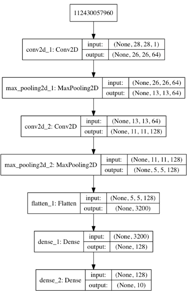
Visualizing a Model’s Structure
You can visualize the model summary using the plot_model function from the module tensorflow.keras.utils:
[35]:fromtensorflow.keras.utilsimportplot_modelfromIPython.displayimportImage plot_model(cnn, to_file='convnet.png', show_shapes=True, show_layer_names=True) Image(filename='convnet.png')
After storing the visualization in convnet.png, we use module IPython.display’s Image class to show the image in the notebook. Keras assigns the layer names in the image:59
59The node with the large integer value 112430057960 at the top of the diagram appears to be a bug in the current version of Keras. This node represents the input layer and should say InputLayer.
Compiling the Model
Once you’ve added all the layers you complete the model by calling its compile method:
[36]: cnn.compile(optimizer='adam',
                  loss='categorical_crossentropy',
                  metrics=['accuracy'])
The arguments are:
optimizer='adam'—The optimizer this model will use to adjust the weights throughout the neural network as it learns. There are many optimizers60—'adam'performs well across a wide variety of models.61,6260For more Keras optimizers, see
https://keras.io/optimizers/.61
https://medium.com/octavian-ai/which-optimizer-and-learning-rate-should-i-use-for-deep-learning-5acb418f9b2.62
https://towardsdatascience.com/types-of-optimization-algorithms-used-in-neural-networks-and-ways-to-optimize-gradient-95ae5d39529f.loss='categorical_crossentropy'—This is the loss function used by the optimizer in multi-classification networks like our convnet, which will predict 10 classes. As the neural network learns, the optimizer attempts to minimize the values returned by the loss function. The lower the loss, the better the neural network is at predicting what each image is. For binary classification (which we’ll use later in this chapter), Keras provides'binary_crossentropy', and for regression,'mean_squared_error'. For other loss functions, seehttps://keras.io/losses/.metrics=['accuracy']—This is a list of the metrics that the network will produce to help you evaluate the model. Accuracy is a commonly used metric in classification models. In this example, we’ll use theaccuracymetric to check the percentage of correct predictions. For a list of other metrics, seehttps://keras.io/metrics/.
15.6.5 Training and Evaluating the Model
Similar to Scikit-learn’s models, we train a Keras model by calling its fit method:
As in Scikit-learn, the first two arguments are the training data and the categorical target labels.
epochsspecifies the number of times the model should process the entire set of training data. As we mentioned earlier, neural networks are trained iteratively.batch_sizespecifies the number of samples to process at a time during each epoch. Most models specify a power of 2 from 32 to 512. Larger batch sizes can decrease model accuracy.63 We chose 64. You can try different values to see how they affect the model’s performance.63Keskar, Nitish Shirish, Dheevatsa Mudigere, Jorge Nocedal, Mikhail Smelyanskiy and Ping Tak Peter Tang. On Large-Batch Training for Deep Learning: Generalization Gap and Sharp Minima. CoRR abs/1609.04836 (2016).
https://arxiv.org/abs/1609.04836.In general, some samples should be used to validate the model. If you specify validation data, after each epoch, the model will use it to make predictions and display the validation loss and accuracy. You can study these values to tune your layers and the
fitmethod’s hyperparameters, or possibly change the layer composition of your model. Here, we used thevalidation_splitargument to indicate that the model should reserve the last 10% (0.1) of the training samples for validation64—in this case, 6000 samples will be used for validation. If you have separate validation data, you can use thevalidation_dataargument (as you’ll see in Section 15.9) to specify a tuple containing arrays of samples and target labels. In general, it’s better to get randomly selected validation data. You can use scikit-learn’strain_test_splitfunction for this purpose (as we’ll do later in this chapter), then pass the randomly selected data with thevalidation_dataargument.64
https://keras.io/getting-started/faq/#how-is-the-validation-split-computed.
In the following output, we highlighted the training accuracy (acc) and validation accuracy (val_acc) in bold:
[37]: cnn.fit(X_train, y_train, epochs=5, batch_size=64,
              validation_split=0.1)
Train on 54000 samples, validate on 6000 samples
Epoch 1/5
54000/54000 [==============================] - 68s 1ms/step   - loss: 0.1407 - acc: 0.9580 - val_loss: 0.0452 - val_acc: 0.9867
Epoch 2/5
54000/54000 [==============================] - 64s 1ms/step   - loss: 0.0426 - acc: 0.9867 - val_loss: 0.0409 - val_acc: 0.9878
Epoch 3/5
54000/54000 [==============================] - 69s 1ms/step   - loss: 0.0299 - acc: 0.9902 - val_loss: 0.0325 - val_acc: 0.9912
Epoch 4/5
54000/54000 [==============================] - 70s 1ms/step   - loss: 0.0197 - acc: 0.9935 - val_loss: 0.0335 - val_acc: 0.9903
Epoch 5/5
54000/54000 [==============================] - 63s 1ms/step   - loss: 0.0155 - acc: 0.9948 - val_loss: 0.0297 - val_acc: 0.9927
[37]: <tensorflow.python.keras.callbacks.History at   0x7f105ba0ada0>
In Section 15.7, we’ll introduce TensorBoard—a TensorFlow tool for visualizing data from your deep-learning models. In particular, we’ll view charts showing how the training and validation accuracy and loss values change through the epochs. In Section 15.8, we’ll demonstrate Andrej Karpathy’s ConvnetJS tool, which trains convnets in your web browser and dynamically visualizes the layers’ outputs, including what each convolutional layer “sees” as it learns. Also run his MNIST and CIFAR10 models. These will help you better understand neural networks’ complex operations.
As the training proceeds, the fit method outputs information showing you the progress of each epoch, how long the epoch took to execute (in this case, each took 63–70 seconds), and the evaluation metrics for that pass. During the last epoch of this model, the accuracy reached 99.48% for the training samples (acc) and 99.27% for the validation samples (val_acc). Those are impressive numbers, given that we have not yet tried to tune the hyperparameters or tweak the number and types of the layers, which could lead to even better (or worse) results. Like machine learning, deep learning is an empirical science that benefits from lots of experimentation.
Evaluating the Model
Now we can check the accuracy of the model on data the model has not yet seen. To do so, we call the model’s model’s evaluate method, which displays as its output, how long it took to process the test samples (four seconds and 366 microseconds in this case):
[38]: loss, accuracy = cnn.evaluate(X_test, y_test)
10000/10000 [==============================] - 4s   366us/step

[39]: loss
[39]: 0.026809450998473768

[40]: accuracy
[40]: 0.9917
According to the preceding output, our convnet model is 99.17% accurate when predicting the labels for unseen data—and, at this point, we have not tried to tune the model. With a little online research, you can find models that can predict MNIST with nearly 100% accuracy. Try experimenting with different numbers of layers, types of layers and layer parameters and observe how those changes affect your results.
Making Predictions
The model’s predict method predicts the classes of the digit images in its argument array (X_test):
[41]: predictions = cnn.predict(X_test)
We can check what the first sample digit should be by looking at y_test[0]:
[42]: y_test[0]
[42]: array([0., 0., 0., 0., 0., 0., 0., 1., 0., 0.],   dtype=float32)
According to this output, the first sample is the digit 7, because the categorical representation of the test sample’s label specifies a 1.0 at index 7—recall that we created this representation via one-hot encoding.
Let’s check the probabilities returned by the predict method for the first test sample:
[43]:forindex, probabilityinenumerate(predictions[0]): print(f'{index}:{probability:.10%}') 0: 0.0000000201% 1: 0.0000001355% 2: 0.0000186951% 3: 0.0000015494% 4: 0.0000000003% 5: 0.0000000012% 6: 0.0000000000% 7: 99.9999761581% 8: 0.0000005577% 9: 0.0000011416%
According to the output, predictions[0] indicates that our model believes this digit is a 7 with nearly 100% certainty. Not all predictions have this level of certainty.
Locating the Incorrect Predictions
Next, we’d like to view some of the incorrectly predicted images to get a sense of the ones our model has trouble with. For example, if it’s always mispredicting 8s, perhaps we need more 8s in our training data.
Before we can view incorrect predictions, we need to locate them. Consider predictions[0] above. To determine whether the prediction was correct, we must compare the index of the largest probability in predictions[0] to the index of the element containing 1.0 in y_test[0]. If these index values are the same, then the prediction was correct; otherwise, it was incorrect. NumPy’s argmax function determines the index of the highest valued element in its array argument. Let’s use that to locate the incorrect predictions. In the following snippet, p is the predicted value array, and e is the expected value array (the expected values are the labels for the dataset’s test images):
[44]: images = X_test.reshape((10000,28,28)) incorrect_predictions = []fori, (p, e)inenumerate(zip(predictions, y_test)): predicted, expected = np.argmax(p), np.argmax(e)ifpredicted != expected: incorrect_predictions.append( (i, images[i], predicted, expected))
In this snippet, we first reshape the samples from the shape (28, 28, 1) that Keras required for learning back to (28, 28), which Matplotlib requires to display the images. Next, we populate the list incorrect_predictions using the for statement. We zip the rows that represent each sample in the arrays predictions and y_test, then enumerate those so we can capture their indexes. If the argmax results for p and e are different, then the prediction was incorrect, and we append a tuple to incorrect_predictions containing that sample’s index, image, the predicted value and the expected value. We can confirm the total number of incorrect predictions (out of 10,000 images in the test set) with:
[45]: len(incorrect_predictions)
[45]: 83
Visualizing Incorrect Predictions
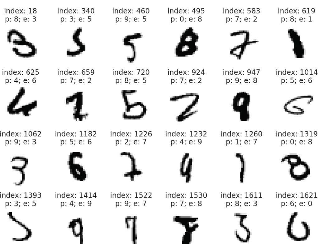
The following snippet displays 24 of the incorrect images labeled with each image’s index, predicted value (p) and expected value (e):
[46]: figure, axes = plt.subplots(nrows=4, ncols=6, figsize=(16,12))foraxes, iteminzip(axes.ravel(), incorrect_predictions): index, image, predicted, expected = item axes.imshow(image, cmap=plt.cm.gray_r) axes.set_xticks([])# remove x-axis tick marksaxes.set_yticks([])# remove y-axis tick marksaxes.set_title( f'index:{index}p:{predicted}; e:{expected}') plt.tight_layout()
Before reading the expected values, look at each digit and write down what digit you think it is. This is an important part of getting to know your data:
Displaying the Probabilities for Several Incorrect Predictions
Let’s look at the probabilities of some incorrect predictions. The following function displays the probabilities for the specified prediction array:
[47]:defdisplay_probabilities(prediction): for index, probabilityinenumerate(prediction): print(f'{index}:{probability:.10%}')
Though the 8 (at index 495) in the first line of the image output looks like an 8, our model had trouble with it. As you can see in the following output, the model predicted this image as a 0, but also thought there was 16% chance it was a 6 and a 23% chance it was an 8:
[48]: display_probabilities(predictions[495])
0: 59.7235262394%
1: 0.0000015465%
2: 0.8047289215%
3: 0.0001740813%
4: 0.0016636326%
5: 0.0030567855%
6: 16.1390662193%
7: 0.0000001781%
8: 23.3022540808%
9: 0.0255270657%
The 2 (at index 583) in the first row was predicted to be a 7 with 62.7% certainty, but the model also thought there was a 36.4% chance it was a 2:
[49]: display_probabilities(predictions[583])
0: 0.0000003016%
1: 0.0000005715%
2: 36.4056706429%
3: 0.0176281916%
4: 0.0000561930%
5: 0.0000000003%
6: 0.0000000019%
7: 62.7455413342%
8: 0.8310816251%
9: 0.0000114385%
The 6 (at index 625) at the beginning of the second row was predicted to be a 4, though that was far from certain. In this case, the probability of a 4 (51.6%) was only slightly higher than the probability of a 6 (48.38%):
[50]: display_probabilities(predictions[625])
0: 0.0008245181%
1: 0.0000041209%
2: 0.0012774357%
3: 0.0000000009%
4: 51.6223073006%
5: 0.0000001779%
6: 48.3754962683%
7: 0.0000000085%
8: 0.0000048182%
9: 0.0000785786%
15.6.6 Saving and Loading a Model
Neural network models can require significant training time. Once you’ve designed and tested a model that suits your needs, you can save its state. This allows you to load it later to make more predictions. Sometimes models are loaded and further trained for new problems. For example, layers in our model already know how to recognize features such as lines and curves, which could be useful in handwritten character recognition (as in the EMNIST dataset) as well. So you could potentially load the existing model and use it as the basis for a more robust model. This process is called transfer learning65,66—you transfer an existing model’s knowledge into a new model. A Keras model’s save method stores the model’s architecture and state information in a format called Hierarchical Data Format (HDF5). Such files use the .h5 file extension by default:
65https://towardsdatascience.com/transfer-learning-from-pre-trained-models-f2393f124751.
66https://medium.com/nanonets/nanonets-how-to-use-deep-learning-when-you-have-limited-data-f68c0b512cab.
[51]: cnn.save('mnist_cnn.h5')
You can load a saved model with the load_model function from the tensorflow.keras.models module:
fromtensorflow.keras.modelsimportload_model
cnn = load_model('mnist_cnn.h5')
You can then invoke its methods. For example, if you’ve acquired more data, you could call predict to make additional predictions on new data, or you could call fit to start training with the additional data.
Keras provides several additional functions that enable you to save and load various aspects of your models. For more information, see
https://keras.io/getting-started/faq/#how-can-i-save-a-keras-model
15.7 Visualizing Neural Network Training with TensorBoard
With deep learning networks, there’s so much complexity and so much going on internally that’s hidden from you that it’s difficult to know and fully understand all the details. This creates challenges in testing, debugging and updating models and algorithms. Deep learning learns the features but there may be enormous numbers of them, and they may not be apparent to you.
Google provides the TensorBoard67,68 tool for visualizing neural networks implemented in TensorFlow and Keras. Just as a car’s dashboard visualizes data from your car’s sensors, such as your speed, engine temperature and the amount of gas remaining, a TensorBoard dashboard visualizes data from a deep learning model that can give you insights into how well your model is learning and potentially help you tune its hyperparameters. Here, we’ll introduce TensorBoard.
67https://github.com/tensorflow/tensorboard/blob/master/README.md.
68https://www.tensorflow.org/guide/summaries_and_tensorboard.
Executing TensorBoard
TensorBoard monitors a folder on your system looking for files containing the data it will visualize in a web browser. Here, you’ll create that folder, execute the TensorBoard server, then access it via a web browser. Perform the following steps:
Change to the
ch15folder in your Terminal, shell or Anaconda Command Prompt.Ensure that your custom Anaconda environment
tf_envis activated:conda activate tf_env
Execute the following command to create a subfolder named
logsin which your deep-learning models will write the information that TensorBoard will visualize:mkdir logs
Execute TensorBoard
tensorboard --logdir=logs
You can now access TensorBoard in your web browser at
http://localhost:6006
If you connect to TensorBoard before executing any models, it will initially display a page indicating “No dashboards are active for the current data set.”69
69TensorBoard does not currently work with Microsofts Edge browser.
The TensorBoard Dashboard
TensorBoard monitors the folder you specified looking for files output by the model during training. When TensorBoard sees updates, it loads the data into the dashboard:

You can view the data as you train or after training completes. The dashboard above shows the TensorBoard SCALARS tab, which displays charts for individual values that change over time, such as the training accuracy (acc) and training loss (loss) shown in the first row, and the validation accuracy (val_acc) and validation_loss (val_loss) shown in the second row. The diagrams visualize a 10-epoch run of our MNIST convnet, which we provided in the notebook MNIST_CNN_TensorBoard.ipynb. The epochs are displayed along the x-axes starting from 0 for the first epoch. The accuracy and loss values are displayed on the y-axes. Looking at the training and validation accuracies, you can see in the first 5 epochs similar results to the five-epoch run in the previous section.
For the 10-epoch run, the training accuracy continued to improve through the 9th epoch, then decreased slightly. This might be the point at which we’re starting to overfit, but we might need to train longer to find out. For the validation accuracy, you can see that it jumped up quickly, then was relatively flat for five epochs before jumping up then decreasing. For the training loss, you can see that it drops quickly, then continuously declines through the ninth epoch, before a slight increase. The validation loss dropped quickly then bounced around. We could run this model for more epochs to see whether results improve, but based on these diagrams, it appears that around the sixth epoch we get a nice combination of training and validation accuracy with minimal validation loss.
Normally these diagrams are stacked vertically in the dashboard. We used the search field (above the diagrams) to show any that had the name “mnist” in their folder name—we’ll configure that in a moment. TensorBoard can load data from multiple models at once and you can choose which to visualize. This makes it easy to compare several different models or multiple runs of the same model.
Copy the MNIST Convnet’s Notebook
To create the new notebook for this example:
Right-click the
MNIST_CNN.ipynbnotebook in JupyterLab’s File Browser tab and select Duplicate to make a copy of the notebook.Right-click the new notebook named
MNIST_CNN-Copy1.ipynb, then select Rename, enter the nameMNIST_CNN_TensorBoard.ipynband press Enter.
Open the notebook by double-clicking its name.
Configuring Keras to Write the TensorBoard Log Files
To use TensorBoard, before you fit the model, you need to configure a TensorBoard object (module tensorflow.keras.callbacks), which the model will use to write data into a specified folder that TensorBoard monitors. This object is known as a callback in Keras. In the notebook, click to the left of snippet that calls the model’s fit method, then type a, which is the shortcut for adding a new code cell above the current cell (use b for below). In the new cell, enter the following code to create the TensorBoard object:
fromtensorflow.keras.callbacksimportTensorBoardimporttime tensorboard_callback = TensorBoard(log_dir=f'./logs/mnist{time.time()}', histogram_freq=1, write_graph=True)
The arguments are:
log_dir—The name of the folder in which this model’s log files will be written. The notation'./logs/'indicates that we’re creating a new folder within the logs folder you created previously, and we follow that with'mnist'and the current time. This ensures that each new execution of the notebook will have its own log folder. That will enable you to compare multiple executions in TensorBoard.histogram_freq—The frequency in epochs that Keras will output to the model’s log files. In this case, we’ll write data to the logs for every epoch.write_graph—When this is true, a graph of the model will be output. You can view the graph in the GRAPHS tab in TensorBoard.
Updating Our Call to fit
Finally, we need to modify the original fit method call in snippet 37. For this example, we set the number of epochs to 10, and we added the callbacks argument, which is a list of callback objects70:
70You can view Kerass other callbacks at https://keras.io/callbacks/.
cnn.fit(X_train, y_train, epochs=10,   batch_size=64,
        validation_split=0.1,   callbacks=[tensorboard_callback])
You can now re-execute the notebook by selecting Kernel > Restart Kernel and Run All Cells in JupyterLab. After the first epoch completes, you’ll start to see data in TensorBoard.
15.8 ConvnetJS: Browser-Based Deep-Learning Training and Visualization
In this section, we’ll overview Andrej Karpathy’s JavaScript-based ConvnetJS tool for training and visualizing convolutional neural networks in your web browser:71
71You also can download ConvnetJS from GitHub at https://github.com/karpathy/convnetjs.
https://cs.stanford.edu/people/karpathy/convnetjs/
You can run the ConvnetJS sample convolutional neural networks or create your own. We’ve used the tool on several desktop, tablet and phone browsers.
The ConvnetJS MNIST demo trains a convolutional neural network using the MNIST dataset we presented in Section 15.6. The demo presents a scrollable dashboard that updates dynamically as the model trains and contains several sections.
Training Stats
This section contains a Pause button that enables you to stop the learning and “freeze” the current dashboard visualizations. Once you pause the demo, the button text changes to resume. Clicking the button again continues training. This section also presents training statistics, including the training and validation accuracy and a graph of the training loss.
Instantiate a Network and Trainer
In this section, you’ll find the JavaScript code that creates the convolutional neural network. The default network has similar layers to the convnet in Section 15.6. The Conv-netJS documentation72 shows the supported layer types and how to configure them. You can experiment with different layer configurations in the provided textbox and begin training an updated network by clicking the change network button.
72https://cs.stanford.edu/people/karpathy/convnetjs/docs.html.
Network Visualization
This key section shows one training image at a time and how the network processes that image through each layer. Click the Pause button to inspect all the layers’ outputs for a given digit to get a sense of what the network “sees” as it learns. The network’s last layer produces the probabilistic classifications. It shows 10 squares—9 black and 1 white, indicating the predicted class of the current digit image.
Example Predictions on Test Set
The final section shows a random selection of the test set images and the top three possible classes for each digit. The one with the highest probability is shown on a green bar and the other two are displayed on red bars. The length of each bar is a visual indication of that class’s probability.
15.9 Recurrent Neural Networks for Sequences; Sentiment Analysis with the IMDb Dataset
In the MNIST CNN network, we focused on stacked layers that were applied sequentially. Non-sequential models are possible, as you’ll see here with recurrent neural networks. In this section, we use Keras’s bundled IMDb (the Internet Movie Database) movie reviews dataset73 to perform binary classification, predicting whether a given review’s sentiment is positive or negative.
73Maas, Andrew L. and Daly, Raymond E. and Pham, Peter T. and Huang, Dan and Ng, Andrew Y. and Potts, Christopher, “Learning Word Vectors for Sentiment Analysis,” Proceedings of the 49th Annual Meeting of the Association for Computational Linguistics: Human Language Technologies, June 2011. Portland, Oregon, USA. Association for Computational Linguistics, pp. 142150. http://www.aclweb.org/anthology/P11-1015.
We’ll use a recurrent neural network (RNN), which processes sequences of data, such as time series or text in sentences. The term “recurrent” comes from the fact that the neural network contains loops in which the output of a given layer becomes the input to that same layer in the next time step. In a time series, a time step is the next point in time. In a text sequence, a “time step” would be the next word in a sequence of words.
The looping in RNNs enables them to learn and remember relationships among the data in the sequence. For example, consider the following sentences we used in the “Natural Language Processing” chapter. The sentence
The food is not good.
clearly has negative sentiment. Similarly, the sentence
The movie was good.
has positive sentiment, though not as positive as
The movie was excellent!
In the first sentence, the word “good” on its own has positive sentiment. However, when preceded by “not,” which appears earlier in the sequence, the sentiment becomes negative. RNNs take into account the relationships among the earlier and later parts of a sequence.
In the preceding example, the words that determined sentiment were adjacent. However, when determining the meaning of text there can be many words to consider and an arbitrary number of words in between them. In this section, we’ll use a Long Short-Term Memory (LSTM) layer, which makes the neural network recurrent and is optimized to handle learning from sequences like the ones we described above.
RNNs have been used for many tasks including:74,75,76
74https://www.analyticsindiamag.com/overview-of-recurrent-neural-networks-and-their-applications/.
75https://en.wikipedia.org/wiki/Recurrent_neural_network#Applications.
76http://karpathy.github.io/2015/05/21/rnn-effectiveness/.
predictive text input—displaying possible next words as you type,
sentiment analysis,
responding to questions with the predicted best answers from a corpus,
inter-language translation, and
automated closed captioning in video.
15.9.1 Loading the IMDb Movie Reviews Dataset
The IMDb movie reviews dataset included with Keras contains 25,000 training samples and 25,000 testing samples, each labeled with its positive (1) or negative (0) sentiment. Let’s import the tensorflow.keras.datasets.imdb module so we can load the dataset:
[1]:fromtensorflow.keras.datasetsimportimdb
The imdb module’s load_data function returns the IMDb training and testing sets. There are over 88,000 unique words in the dataset. The load_data function enables you to specify the number of unique words to import as part of the training and testing data. In this case, we loaded only the top 10,000 most frequently occurring words due to the memory limitations of our system and the fact that we’re (intentionally) training on a CPU rather than a GPU (because most of our readers will not have access to systems with GPUs and TPUs). The more data you load, the longer training will take, but more data may help produce better models:
[2]: number_of_words = 10000

[3]: (X_train, y_train), (X_test, y_test) = imdb.load_data(
         num_words=number_of_words)
The load_data function returns a tuple of two elements containing the training and testing sets. Each element is itself a tuple containing the samples and labels, respectively. In a given review, load_data replaces any words outside the top 10,000 with a placeholder value, which we’ll discuss shortly.
15.9.2 Data Exploration
Let’s check the dimensions of the training set samples (X_train), training set labels (y_train), testing set samples (X_test) and testing set labels (y_test):
[4]: X_train.shape
[4]: (25000,)

[5]: y_train.shape
[5]: (25000,)

[6]: X_test.shape
[6]: (25000,)

[7]: y_test.shape
[7]: (25000,)
The arrays y_train and y_test are one-dimensional arrays containing 1s and 0s, indicating whether each review is positive or negative. Based on the preceding outputs, X_train and X_test also appear to be one-dimensional. However, their elements actually are lists of integers, each representing one review’s contents, as shown in snippet [9]:77
77Here we used the %pprint magic to turn off pretty printing so the following snippets output could be displayed horizontally rather than vertically to save space. You can turn pretty printing back on by re-executing the %pprint magic.
[8]: %pprint
[8]: Pretty printing has been turned OFF

[9]: X_train[123]
[9]: [1, 307, 5, 1301, 20, 1026, 2511, 87, 2775, 52, 116,   5, 31, 7, 4, 91, 1220, 102, 13, 28, 110, 11, 6, 137, 13, 115, 219, 141, 35,   221, 956, 54, 13, 16, 11, 2714, 61, 322, 423, 12, 38, 76, 59, 1803, 72, 8, 2,   23, 5, 967, 12, 38, 85, 62, 358, 99]
Keras deep learning models require numeric data, so the Keras team preprocessed the IMDb dataset for you.
Movie Review Encodings
Because the movie reviews are numerically encoded, to view their original text, you need to know the word to which each number corresponds. Keras’s IMDb dataset provides a dictionary that maps the words to their indexes. Each word’s corresponding value is its frequency ranking among all the words in the entire set of reviews. So the word with the ranking 1 is the most frequently occurring word (calculated by the Keras team from the dataset), the word with ranking 2 is the second most frequently occurring word, and so on.
Though the dictionary values begin with 1 as the most frequently occurring word, in each encoded review (like X_train[123] shown previously), the ranking values are offset by 3. So any review containing the most frequently occurring word will have the value 4 wherever that word appears in the review. Keras reserves the values 0, 1 and 2 in each encoded review for the following purposes:
The value 0 in a review represents padding. Keras deep learning algorithms expect all the training samples to have the same dimensions, so some reviews may need to be expanded to a given length and some shortened to that length. Reviews that need to be expanded are padded with 0s.
The value 1 represents a token that Keras uses internally to indicate the start of a text sequence for learning purposes.
The value 2 in a review represents an unknown word—typically a word that was not loaded because you called
load_datawith thenum_wordsargument. In this case, any review that contained words with frequency rankings greater thannum_wordswould have those words’ numeric values replaced with 2. This is all handled by Keras when you load the data.
Because each review’s numeric values are offset by 3, we’ll have to account for this when we decode the review.
Decoding a Movie Review
Let’s decode a review. First, get the word-to-index dictionary by calling the function get_word_index from the tensorflow.keras.datasets.imdb module:
[10]: word_to_index = imdb.get_word_index()
The word 'great' might appear in a positive movie review, so let’s see whether it’s in the dictionary:
[11]: word_to_index['great']
[11]: 84
According to the output, 'great' is the dataset’s 84th most frequent word. If you look up a word that’s not in the dictionary, you’ll get an exception.
To transform the frequency ratings into words, let’s first reverse the word_to_index dictionary’s mapping, so we can look up every word by its frequency rating. The following dictionary comprehension reverses the mapping:
[12]: index_to_word =
          {index: word for   (word, index) in word_to_index.items()}
Recall that a dictionary’s items method enables us to iterate through tuples of key–value pairs. We unpack each tuple into the variables word and index, then create an entry in the new dictionary with the expression index: word.
The following list comprehension gets the top 50 words from the new dictionary—recall that the most frequent word has the value 1:
[13]: [index_to_word[i]foriinrange(1,51)] [13]: ['the', 'and', 'a', 'of', 'to', 'is', 'br', 'in', 'it', 'i', 'this', 'that', 'was', 'as', 'for', 'with', 'movie', 'but', 'film', 'on', 'not', 'you', 'are', 'his', 'have', 'he', 'be', 'one', 'all', 'at', 'by', 'an', 'they', 'who', 'so', 'from', 'like', 'her', 'or', 'just', 'about', "it's", 'out', 'has', 'if', 'some', 'there', 'what', 'good', 'more']
Note that most of these are stop words. Depending on the application, you might want to remove or keep the stop words. For example, if you were creating a predictive-text application that suggests the next word in a sentence the user is typing, you’d want to keep the stop words so they can be displayed as predictions.
Now, we can decode a review. We use the index_to_word dictionary’s two-argument method get rather than the [] operator to get value for each key. If a value is not in the dictionary, the get method returns its second argument, rather than raising an exception. The argument i - 3 accounts for the offset in the encoded reviews of each review’s frequency ratings. When the Keras reserved values 0–2 appear in a review, get returns '?'; otherwise, get returns the word with the key i - 3 in the index_to_word dictionary:
[14]:' '.join([index_to_word.get(i -3,'?')foriinX_train[123]]) [14]: '? beautiful and touching movie rich colors great settings good acting and one of the most charming movies i have seen in a while i never saw such an interesting setting when i was in china my wife liked it so much she asked me to ? on and rate it so other would enjoy too'
We can see from the y_train array that this review is classified as positive:
[15]: y_train[123]
[15]: 1
15.9.3 Data Preparation
The number of words per review varies, but the Keras requires all samples to have the same dimensions. So, we need to perform some data preparation. In this case, we need to restrict every review to the same number of words. Some reviews will need to be padded with additional data and others will need to be truncated. The pad_sequences utility function (module tensorflow.keras.preprocessing.sequence) reshapes X_train’s samples (that is, its rows) to the number of features specified by the maxlen argument (200) and returns a two-dimensional array:
[16]: words_per_review =200[17]:fromtensorflow.keras.preprocessing.sequenceimportpad_sequences [18]: X_train = pad_sequences(X_train, maxlen=words_per_review)
If a sample has more features, pad_sequences truncates it to the specified length. If a sample has fewer features, pad_sequences adds 0s to the beginning of the sequence to pad it to the specified length. Let’s confirm X_train’s new shape:
[19]: X_train.shape
[19]: (25000, 200)
We also must reshape X_test for later in this example when we evaluate the model:
[20]: X_test = pad_sequences(X_test,   maxlen=words_per_review)

[21]: X_test.shape
[21]: (25000, 200)
Splitting the Test Data into Validation and Test Data
In our convnet, we used the fit method’s validation_split argument to indicate that 10% of our training data should be set aside to validate the model as it trains. For this example, we’ll manually split the 25,000 test samples into 20,000 test samples and 5,000 validation samples. We’ll then pass the 5,000 validation samples to the model’s fit method via the argument validation_data. Let’s use Scikit-learn’s train_test_split function from the previous chapter to split the test set:
[22]:fromsklearn.model_selectionimporttrain_test_split X_test, X_val, y_test, y_val = train_test_split( X_test, y_test, random_state=11, test_size=0.20)
Let’s also confirm the split by checking X_test’s and X_val’s shapes:
[23]: X_test.shape
[23]: (20000, 200)

[24]: X_val.shape
[24]: (5000, 200)
15.9.4 Creating the Neural Network
Next, we’ll configure the RNN. Once again, we begin with a Sequential model to which we’ll add the layers that compose our network:
[25]:fromtensorflow.keras.modelsimportSequential [26]: rnn = Sequential()
Next, let’s import the layers we’ll use in this model:
[27]:fromtensorflow.keras.layersimportDense, LSTM [28]:fromtensorflow.keras.layers.embeddingsimportEmbedding
Adding an Embedding Layer
Previously, we used one-hot encoding to convert the MNIST dataset’s integer labels into categorical data. The result for each label was a vector in which all but one element was 0. We could do that for the index values that represent our words. However, this example processes 10,000 unique words. That means we’d need a 10,000-by-10,000 array to represent all the words. That’s 100,000,000 elements, and almost all the array elements would be 0. This is not an efficient way to encode the data. If we were to process all 88,000+ unique words in the dataset, we’d need an array of nearly eight billion elements!
To reduce dimensionality, RNNs that process text sequences typically begin with an embedding layer that encodes each word in a more compact dense-vector representation. The vectors produced by the embedding layer also capture the word’s context—that is, how a given word relates to the words around it. So the embedding layer enables the RNN to learn word relationships among the training data.
There are also predefined word embeddings, such as Word2Vec and GloVe. You can load these into neural networks to save training time. They’re also sometimes used to add basic word relationships to a model when smaller amounts of training data are available. This can improve the model’s accuracy by allowing it to build upon previously learned word relationships, rather than trying to learn those relationships with insufficient amounts of data.
Let’s create an Embedding layer (module tensorflow.keras.layers):
[29]: rnn.add(Embedding(input_dim=number_of_words,   output_dim=128,
                        input_length=words_per_review))
The arguments are:
input_dim—The number of unique words.output_dim—The size of each word embedding. If you load pre-existing embeddings78 like Word2Vec and GloVe, you must set this to match the size of the word embeddings you load.78
https://blog.keras.io/using-pre-trained-word-embeddings-in-a-keras-model.html.input_length=words_per_review—The number of words in each input sample.
Adding an LSTM Layer
Next, we’ll add an LSTM layer:
[30]: rnn.add(LSTM(units=128, dropout=0.2, recurrent_dropout=0.2))
The arguments are:
units—The number of neurons in the layer. The more neurons the more the network can remember. As a guideline, you can start with a value between the length of the sequences you’re processing (200 in this example) and the number of classes you’re trying to predict (2 in this example).7979
https://towardsdatascience.com/choosing-the-right-hyperparameters-for-a-simple-lstm-using-keras-f8e9ed76f046.dropout—The percentage of neurons to randomly disable when processing the layer’s input and output. Like the pooling layers in our convnet, dropout is a proven technique80,81 that reduces overfitting. Keras provides aDropoutlayer that you can add to your models.80Yarin, Ghahramani, and Zoubin. A Theoretically Grounded Application of Dropout in Recurrent Neural Networks. October 05, 2016.
https://arxiv.org/abs/1512.05287.81Srivastava, Nitish, Geoffrey Hinton, Alex Krizhevsky, Ilya Sutskever, and Ruslan Salakhutdinov. Dropout: A Simple Way to Prevent Neural Networks from Overfitting. Journal of Machine Learning Research 15 (June 14, 2014): 1929-1958.
http://jmlr.org/papers/volume15/srivastava14a/srivastava14a.pdf.recurrent_dropout—The percentage of neurons to randomly disable when the layer’s output is fed back into the layer again to allow the network to learn from what it has seen previously.
The mechanics of how the LSTM layer performs its task are beyond the scope of this book. Chollet says: “you don’t need to understand anything about the specific architecture of an LSTM cell; as a human, it shouldn’t be your job to understand it. Just keep in mind what the LSTM cell is meant to do: allow past information to be reinjected at a later time.”82
82Chollet, François. Deep Learning with Python. p. 204. Shelter Island, NY: Manning Publications, 2018.
Adding a Dense Output Layer
Finally, we need to take the LSTM layer’s output and reduce it to one result indicating whether a review is positive or negative, thus the value 1 for the units argument. Here we use the 'sigmoid' activation function, which is preferred for binary classification.83 It reduces arbitrary values into the range 0.0–1.0, producing a probability:
83Chollet, François. Deep Learning with Python. p.114. Shelter Island, NY: Manning Publications, 2018.
[31]: rnn.add(Dense(units=1, activation='sigmoid'))
Compiling the Model and Displaying the Summary
Next, we compile the model. In this case, there are only two possible outputs, so we use the binary_crossentropy loss function:
[32]: rnn.compile(optimizer='adam',
                  loss='binary_crossentropy',
                  metrics=['accuracy'])
The following is the summary of our model. Notice that even though we have fewer layers than our convnet, the RNN has nearly three times as many trainable parameters (the network’s weights) as the convnet and more parameters means more training time. The large number of parameters primarily comes from the number of words in the vocabulary (we loaded 10,000) times the number of neurons in the Embedding layer’s output (128):
[33]: rnn.summary()
_________________________________________________________________
Layer (type)                 Output Shape                Param #
=================================================================
embedding_1 (Embedding)      (None, 200, 128)            1280000
_________________________________________________________________
lstm_1 (LSTM)                (None, 128)                 131584
_________________________________________________________________
dense_1 (Dense)              (None, 1)                   129
=================================================================
Total params: 1,411,713
Trainable params: 1,411,713
Non-trainable params: 0
15.9.5 Training and Evaluating the Model
Let’s train our model.84 Notice for each epoch that the model takes significantly longer to train than our convnet did. This is due to the larger numbers of parameters (weights) our RNN model needs to learn. We bolded the accuracy (acc) and validation accuracy (val_acc) values for readability—these represent the percentage of training samples and the percentage of validation_data samples that the model predicts correctly.
84At the time of this writing, TensorFlow displayed a warning when we executed this statement. This is a known TensorFlow issue and, according to the forums, you can safely ignore the warning.
[34]: rnn.fit(X_train, y_train, epochs=10, batch_size=32,
              validation_data=(X_test, y_test))
Train on 25000 samples, validate on 5000 samples
Epoch 1/5
25000/25000 [==============================] - 299s   12ms/step - loss: 0.6574 - acc: 0.5868 - val_loss:   0.5582 - val_acc: 0.6964
Epoch 2/5
25000/25000 [==============================] - 298s   12ms/step - loss: 0.4577 - acc: 0.7786   - val_loss: 0.3546 - val_acc: 0.8448
Epoch 3/5
25000/25000 [==============================] - 296s   12ms/step - loss: 0.3277 - acc: 0.8594   - val_loss: 0.3207 - val_acc: 0.8614
Epoch 4/5
25000/25000 [==============================] - 307s   12ms/step - loss: 0.2675 - acc: 0.8864 - val_loss:   0.3056 - val_acc: 0.8700
Epoch 5/5
25000/25000 [==============================] - 310s   12ms/step - loss: 0.2217 - acc: 0.9083   - val_loss: 0.3264 - val_acc: 0.8704
[34]: <tensorflow.python.keras.callbacks.History object   at 0xb3ba882e8>
Finally, we can evaluate the results using the test data. Function evaluate returns the loss and accuracy values. In this case, the model was 85.99% accurate:
[35]: results = rnn.evaluate(X_test, y_test)
20000/20000 [==============================] - 42s 2ms/step

[36]: results
[36]: [0.3415240607559681, 0.8599]
Note that the accuracy of this model seems low compared to our MNIST convnet’s results, but this is a much more difficult problem. If you search online for other IMDb sentiment-analysis binary-classification studies, you’ll find lots of results in the high 80s. So we did reasonably well with our small recurrent neural network of only three layers. You might want to study some online models and try to produce a better model.
15.10 Tuning Deep Learning Models
In Section 15.9.5, notice in the fit method’s output that both the testing accuracy (85.99%) and validation accuracy (87.04%) were significantly less than the 90.83% training accuracy. Such disparities are usually the result of overfitting, so there is plenty of room for improvement in our model.85,86 If you look at the output of each epoch, you’ll notice both the training and validation accuracy continue to increase. Recall that training for too many epochs can lead to overfitting, but it’s possible we have not yet trained enough. Perhaps one hyperparameter tuning option for this model would be to increase the number of epochs.
85https://towardsdatascience.com/deep-learning-overfitting-846bf5b35e24.
86https://hackernoon.com/memorizing-is-not-learning-6-tricks-to-prevent-overfitting-in-machine-learning-820b091dc42.
Some variables that affect your models’ performance include:
having more or less data to train with
having more or less to test with
having more or less to validate with
having more or fewer layers
the types of layers you use
the order of the layers
In our IMDb RNN example, some things we could tune include:
trying different amounts of the training data—we used only the top 10,000 words
different numbers of words per review—we used only 200,
different numbers of neurons in our layers,
more layers or
possibly loading pre-trained word vectors rather than having our Embedding layer learn them from scratch.
The compute time required to train models multiple times is significant so, in deep learning, you generally do not tune hyperparameters with techniques like k-fold cross-validation or grid search.87 There are various tuning techniques,88,89,90,91 but one particularly promising area is automated machine learning (AutoML). For example, the Auto-Keras92 library is specifically geared to automatically choosing the best configurations for your Keras models. Google’s Cloud AutoML and Baidu’s EZDL are among various other automated machine learning efforts.
87https://www.quora.com/Is-cross-validation-heavily-used-in-deep-learning-or-is-it-too-expensive-to-be-used.
88https://towardsdatascience.com/what-are-hyperparameters-and-how-to-tune-the-hyperparameters-in-a-deep-neural-network-d0604917584a.
89https://medium.com/machine-learning-bites/deeplearning-series-deep-neural-networks-tuning-and-optimization-39250ff7786d.
90https://flyyufelix.github.io/2016/10/03/fine-tuning-in-keras-part1.html and https://flyyufelix.github.io/2016/10/08/fine-tuning-in-keras-part2.html.
91https://towardsdatascience.com/a-comprehensive-guide-on-how-to-fine-tune-deep-neural-networks-using-keras-on-google-colab-free-daaaa0aced8f.
15.11 Convnet Models Pretrained on ImageNet
With deep learning, rather than starting fresh on every project with costly training, validating and testing, you can use pretrained deep neural network models to:
make new predictions,
continue training them further with new data or
transfer the weights learned by a model for a similar problem into a new model—this is called transfer learning.
Keras Pretrained Convnet Models
Keras comes bundled with the following pretrained convnet models,93 each pretrained on Image-Net94—a growing dataset of 14+ million images:
93https://keras.io/applications/.
Xception
VGG16
VGG19
ResNet50
Inception v3
Inception-ResNet v2
MobileNet v1
DenseNet
NASNet
MobileNet v2
Reusing Pretrained Models
ImageNet is too big for efficient training on most computers, so most people interested in using it start with one of the smaller pretrained models.
You can reuse just the architecture of each model and train it with new data, or you can reuse the pretrained weights. For a few simple examples, see:
https://keras.io/applications/ImageNet Challenge
In the end-of-chapter projects, you’ll research and use some of these bundled models. You’ll also investigate the ImageNet Large Scale Visual Recognition Challenge for evaluating object-detection and image-recognition models.95 This competition ran from 2010 through 2017. ImageNet now has a continuously running challenge on the Kaggle competition site called the ImageNet Object Localization Challenge.96 The goal is to identify “all objects within an image, so those images can then be classified and annotated.” ImageNet releases the current participants leaderboard once per quarter.
95http://www.image-net.org/challenges/LSVRC/.
96https://www.kaggle.com/c/imagenet-object-localization-challenge.
A lot of what you’ve seen in the machine learning and deep learning chapters is what the Kaggle competition website is all about. There’s no obvious optimal solution for many machine learning and deep learning tasks. People’s creativity is really the only limit. On Kaggle, companies and organizations fund competitions where they encourage people worldwide to develop better-performing solutions than they’ve been able to do for something that’s important to their business or organization. Sometimes companies offer prize money, which has been as high as $1,000,000 on the famous Netflix competition. Netflix wanted to get a 10% or better improvement in their model for determining whether people will like a movie, based on how they rated previous ones.97 They used the results to help make better recommendations to members. Even if you do not win a Kaggle competition, it’s a great way to get experience working on problems of current interest.
97https://netflixprize.com/rules.html.
15.12 Wrap-Up
In Chapter 16, you peered into the future of AI. Deep Learning has captured the imagination of the computer-science and data science-communities. This may be the most important AI chapter in the book.
We mentioned the key deep-learning platforms, indicating that Google’s TensorFlow is the most widely used. We discussed why Keras, which presents a friendly interface to TensorFlow, has become so popular.
We set up a custom Anaconda environment for TensorFlow, Keras and JupyterLab, then used the environment to implement the Keras examples.
We explained what tensors are and why they’re crucial to deep learning. We discussed the basics of neurons and multi-layered neural networks for building Keras deep-learning models. We considered some popular types of layers and how to order them.
We introduced convolutional neural networks (convnets) and indicated that they’re especially appropriate for computer-vision applications. We then built, trained, validated and tested a convnet using the MNIST database of handwritten digits for which we achieved 99.17% prediction accuracy. This is remarkable, given that we achieved it by working with a only a basic model and without doing any hyperparameter tuning. You can try more sophisticated models and tune the hyperparameters to try to achieve better performance. We listed a variety of intriguing computer vision tasks.
We introduced TensorBoard for visualizing TensorFlow and Keras neural network training and validation. We also discussed ConvnetJS, a browser-based convnet training and visualization tool, which enables you to peek inside the training process.
Next, we presented recurrent neural networks (RNNs) for processing sequences of data, such as time series or text in sentences. We used an RNN with the IMDb movie reviews dataset to perform binary classification, predicting whether each review’s sentiment was positive or negative. We also discussed tuning deep learning models and how high-performance hardware, like NVIDIA’s GPUs and Google’s TPUs, is making it possible for more people to tackle more substantial deep-learning studies.
Given how costly and time-consuming it is to train deep-learning models, we explained the strategy of using pretrained models. We listed various Keras convnet image-processing models that were trained on the massive ImageNet dataset, and discussed how transfer learning enables you to use these models to create new ones quickly and effectively. Deep learning is a large, complex topic. We focused on the basics in the chapter.
In the next chapter, we present the big data infrastructure that supports the kinds of AI technologies we’ve discussed in Chapters 12 through 15. We’ll consider the Hadoop and Spark platforms for big data batch processing and real-time streaming applications. We’ll look at relational databases and the SQL language for querying them—these have dominated the database field for many decades. We’ll discuss how big data presents challenges that relational databases don’t handle well, and consider how NoSQL databases are designed to handle those challenges. We’ll conclude the book with a discussion of the Internet of Things (IoT), which will surely be the world’s largest big-data source and will present many opportunities for entrepreneurs to develop leading-edge businesses that will truly make a difference in people’s lives.